Flowchart, AI, Deep Learning, Medicine, n2value

Are computers better than doctors ? Will the computer see you now ? What we learnt from the ChexNet paper for pneumonia diagnosis …

Author’s Note: This was a fun side-project for the American College of Radiology’s Residents and Fellows Section.  Judy Gichoya and I co-wrote the article.   The original article was posted by Judy to Medium and appeared on HackerNoon.  It was really an enlightening gathering of experts in the field.  There is a small, but hopefully growing number of radiologists who are also deep learning practitioners.


Written by Judy Gichoya & Stephen Borstelmann MD


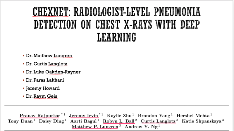
In December 2017 , we (radiologists both in training, staff radiologists and AI practitioners) discussed our role as knowledge experts in world of AI, summarized here https://becominghuman.ai/radiologists-as-knowledge-experts-in-a-world-of-artificial-intelligence-summary-of-radiology-ec63a7002329. For the month of January, we addressed the performance of deep learning algorithms for disease diagnosis , specifically focusing on the paper by the stanford group — CheXNet: Radiologist-Level Pneumonia Detection on Chest X-Rays with Deep Learning. We continue to generate a large interest in the journal club , with 347 people registered , 150 of whom signed on January 24th 2018 to participate in the discussion.

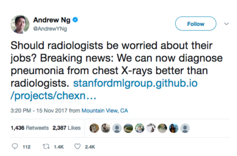
The paper has had 3 revisions and is available here https://arxiv.org/abs/1711.05225 . Like many deep learning papers that claim super human performance , the paper was widely circulated in the news media, several blog posts , on reddit and twitter.

ngtwitter

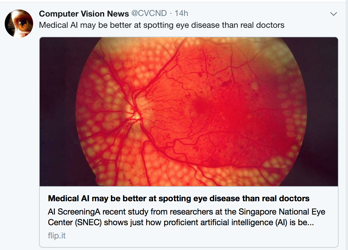
Please note that the findings of superhuman performance are increasingly being reported in medical AI papers. For example, this article denotes that “Medical AI May Be Better at Spotting Eye Disease Than Real Doctors”

CVDretina

To help critique the ChexNet paper , we constituted a panel composed of the author team (most of the authors listed on the paper were kind enough to be in attendance — thank you!), Dr. Luke(blog) and Dr. Paras (blog) who had critiqued the data used and Jeremy Howard (past president and chief scientist of Kaggle, a data analytics competition site, Ex-CEO of Enlitic, a healthcare imaging company, and the Current CEO of Fast.ai, a deep learning educational site) to provide insight to deep learning methodology.

chexnet

In this blog we summarise the methodology of reviewing medical AI papers.

Radiology 101

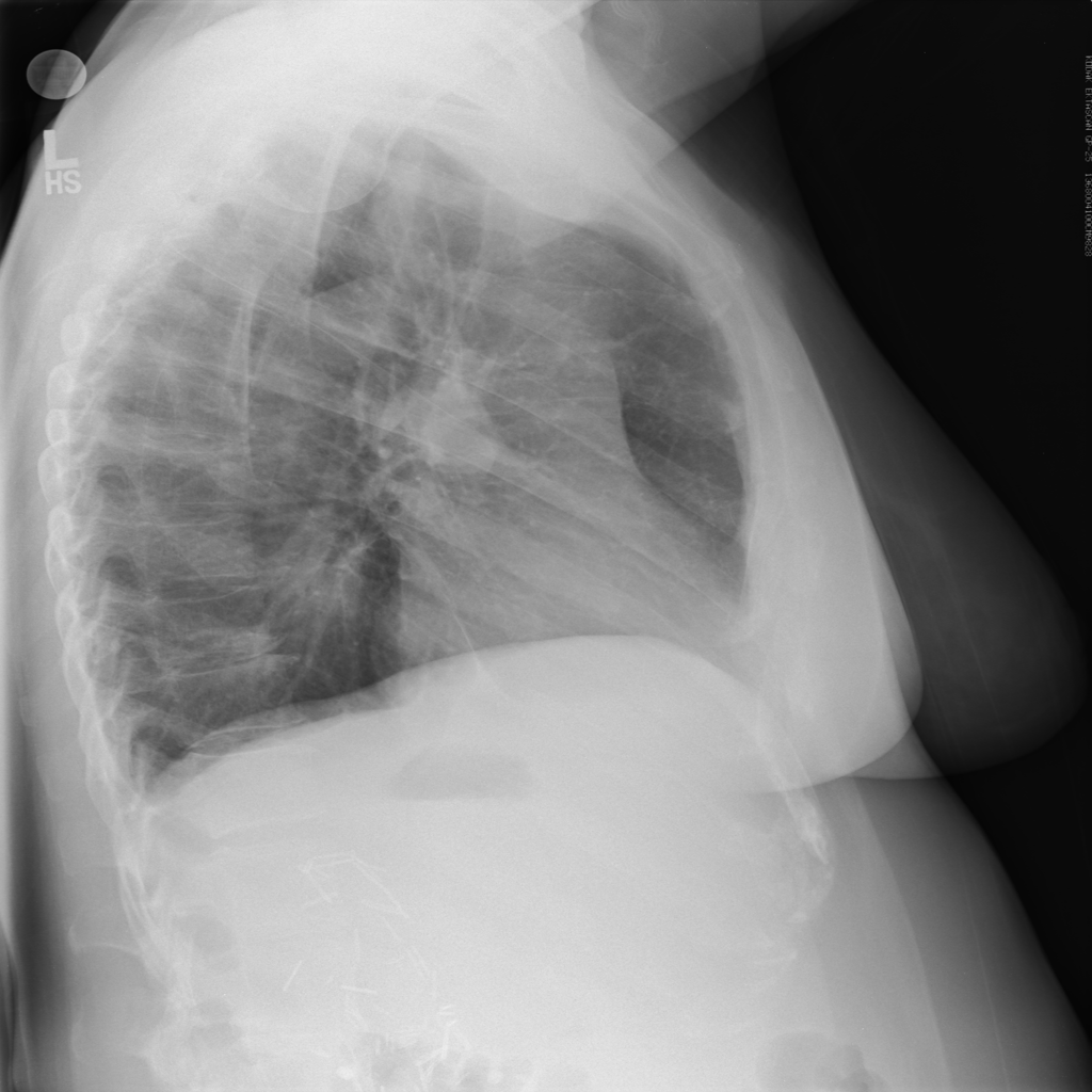
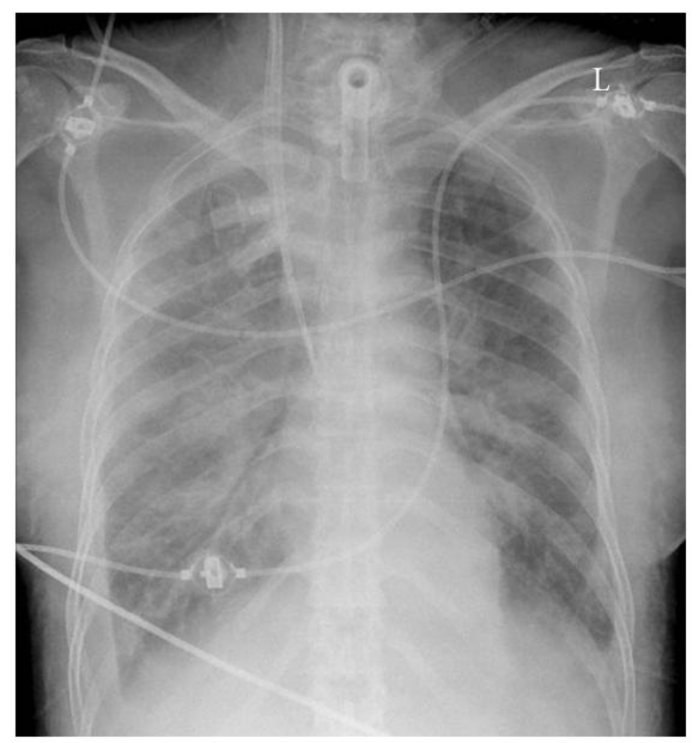
The ChexNet paper reviews performance of AI versus 4 trained radiologists in diagnosing pneumonia. Pneumonia is a clinical diagnosis — a patient will present with fever and cough , and can get a chest Xray(CXR) to identify complications of pneumonia. Patients will usually get blood cultures to supplement diagnosis. Pneumonia on a CXR is not easily distinguishable from other findings that fill the alevolar spaces — specifically pus , blood , fluid or collapsed lung called atelectasis. The radiologists interpreting these studies can therefore use terms like infiltrates , consolidation and atelectasis interchangeably.

Show me the data

The data used for this study is the ChestX-ray14 dataset which is the largest publicly available imaging data set that consists of 112,120 frontal chext xray radiographs of 30,805 unique patients and expands the ChestX-Ray 8, described by Wang, et. al. Each radiograph is labeled with one or more of 14 different pathology labels, or a ‘no finding’ label.

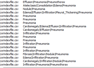
Labeling of the radiographs was performed using Natural Language Processing (NLP) by mining the text in the radiology reports. Individual case labels were not assigned by humans.

Critique: Labeling medical data remains a big challenge especially because the radiology report is a tool for communicating to ordering doctors and not a description of the images. For example , in an ICU film with a central line, tracheostomy tube and chest tube may be reported as “stable lines and tubes” without detailed description of the every individual finding on the CXR. This can be missclassified by NLP as a study without findings. This image-report disconcordance occurs at a high rate on this dataset.

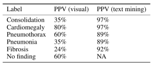
Moreover reportable findings could be ignored by the NLP technique and/or labeling schema, either through error or pathology outside of one of the 14 labels. The paper’s claims of 90%+ NLP mining accuracy do not appear to be accurate. (SMB,LOR,JH). One of the panelists — Luke reviewed several hundred examples and found the NLP labeling about 50% accurate overall compared to the image, with the pneumonia labeling worse — 30–40%.

Jeremy Howard notes that the use of an old NLP tool contributes to the inaccuracy due to the preponderance of ‘No Findings’ cases in the dataset skewing the data — he doesn’t think that the precision of normal findings in this dataset is likely improved over random. Looking at the pneumonia label, it is only 60% accurate. A lot of the discrepancy can be drawn back to the core NLP method, which he characterized as “massively out of date and known to be inaccurate”. He feels a re-characterization of the labels with a more up-to-date NLP system is appropriate.

Chest X Ray, CXR, Deep Learning, CheXNet, n2value, tracheostomy, infiltrates, pulmonary edema
Chest Xray showing a tracheostomy tube , right internal jugular dialysis line and diffuse infiltrates likely pulmonary edema. The lines and tubes for an ICU patient are easily reported as “Stable”

The stanford group tackled the labeling challenge by having 4 radiologists (one specializing in thoracic imaging and 3 non thoracic radiologists) assign labels to a subset of the data for training created through a stratified random sampling, for a minimum of 50 positive cases of each label, with a final N=420.

Critique: The ChestXRay14 contains many patients with only one radiograph but those who had multiple studies tended to have many. While the text-mined reports may match clinical information, any mismatch between the assigned label and radiographic appearance hurts the predictive power of the dataset.

Moreover , what do the labels actually mean? Dr. Oakden-Rayner questions what the labels mean — do they mean a radiologic pneumonia or a clinical pneumonia? In an immunocompromised patient, radiography of a pneumonia might be negative, largely because the patient cannot mount an immune response to the pathogen. This does not mean that the clinical diagnosis of pneumonia is inaccurate. The imaging appearance and clinical appearance/diagnosis therefore would not match.

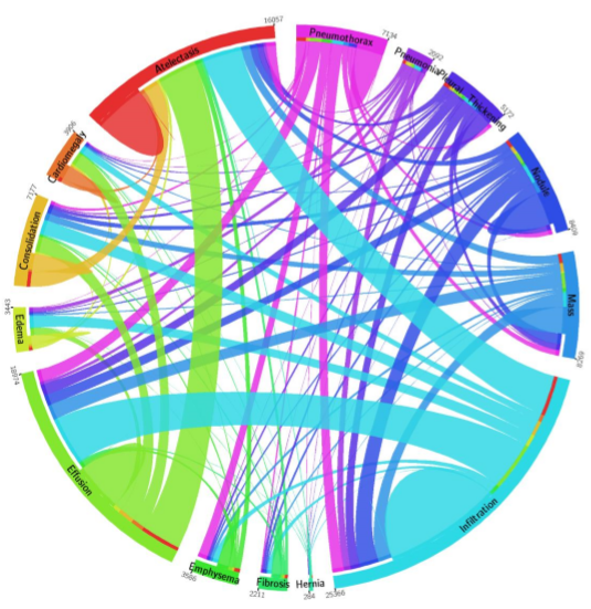
The closeness of four of the labels: Pneumonia, Consolidation, Infiltration, and Atelectasis introduces a new level of complexity. Pneumonia is a subset of consolidation and infiltration is a superset of consolidation. While the dataset labels these as 4 separate entities, to the radiologic practitioner they may not be separate at all. It is important to have experts look at images when doing an image classification task.

See a great summary of the data problems on this blog posting from Luke who was one of the panelists here.
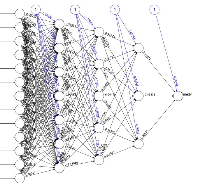
Model

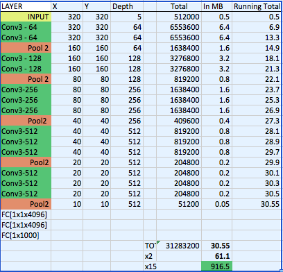
The CheXNet algorithm is a 121-layer deep 2D Convolutional Neural Network; a Densenet after Huang & Liu. The Densenet’s multiple residual connections reduce parameters and training time, allowing a deeper, more powerful model. The model accepts a vectorized two-dimensional image of size 224 pixels by 224 pixels.

DenseNet, Convolutional Neural Network, CNN, AI, machine learning, deep learning
Densenet

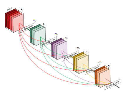
To improve trust in CheXNet’s output, a Class Activation Mapping (GRAD-CAM) heatmap was utilized after Zhou et al. This allows the human user to “see” what areas of the radiograph provide the strongest activation of the Densenet for the highest probability label.

Critique: Jeremy notes that image preprocessing of resizing to 224×224 pixel size images and adding random horizontal flips is fairly standard, but leaves room for potential improvement, as effective data augmentation is one of the best ways to improve a model. Image downsizing to 224×224 is a known issue — both from research and practical experience at Enlitic, larger images perform better in medical imaging (SMB: Multiple top 5 winners of the 2017 RSNA Bone age challenge had image sizes near 512×512). Mr. Howard feels there is no reason to leave Imagenet trained models this size any longer. Regarding the model choice, the Densenet model is adequate, but NasNets in the last 12 months have shown significant improvement (50%) over older models.

Pre-trained Imagenet weights were used, which is fine & a standard approach; but Jeremy felt it would be nice if we had a medical imagenet for some semi-supervised training of an AutoML encoder or a siamese network to cross validate patients — leaving room for improvement. Consider that Imagenet consists of color images of dogs, cats, planes and trains — and we are getting great results on X-rays? While better than nothing, ANY pretrained network trained on medical images in any modality would probably perform superiorly.

The Stanford team’s best idea was to train on multiple labels at the same time — it is best to build a single model that predicts multiple classes — counterintuitive, but bears out in deep learning models, and likely responsible for their model yielding better results than prior studies. The more classes you train the model on properly, the better results you can expect.

Results

F1 scores were used to evaluate both CheXNet model and the Stanford Radiologists.

Precision, Recall, F1 Score, ROC, AUC, AUCROC, metrics, measure, n2value
Calculating F1 score

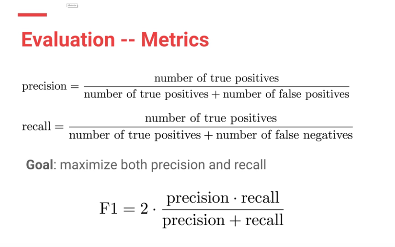
Each Radiologists’ F1 score was calculated by considering the other three radiologists as “ground truth.” ChexNet’s F1 score, was calculated vs. all 4 radiologists. A bootstrap calculation was added to yield 95% confidence intervals.

CheXnet’s results are as follows:Evaluation-results

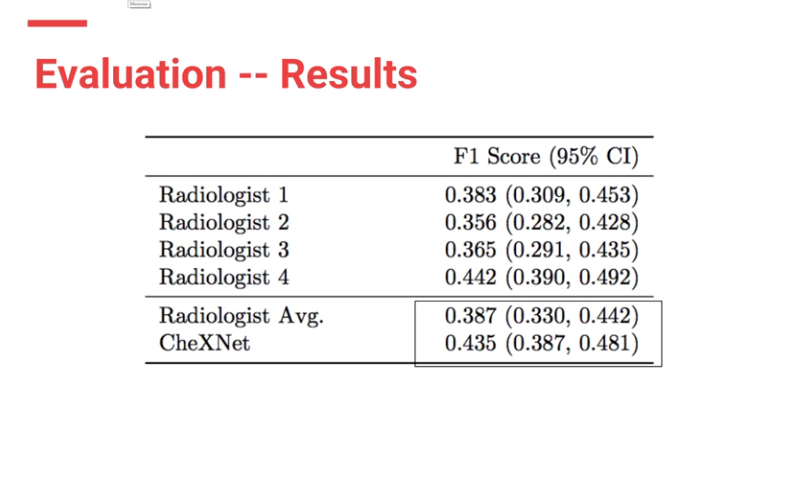
From the results, ChexNet outperforms human radiologists. The varying F1 scores can be interpreted to imply that for each study , 4 radiologists do not seem to agree with each other on findings. However there is an outlier (rad 4 — with an F score of 0.442) who is the thoracic trained radiologists who performs better than the ChexNet.

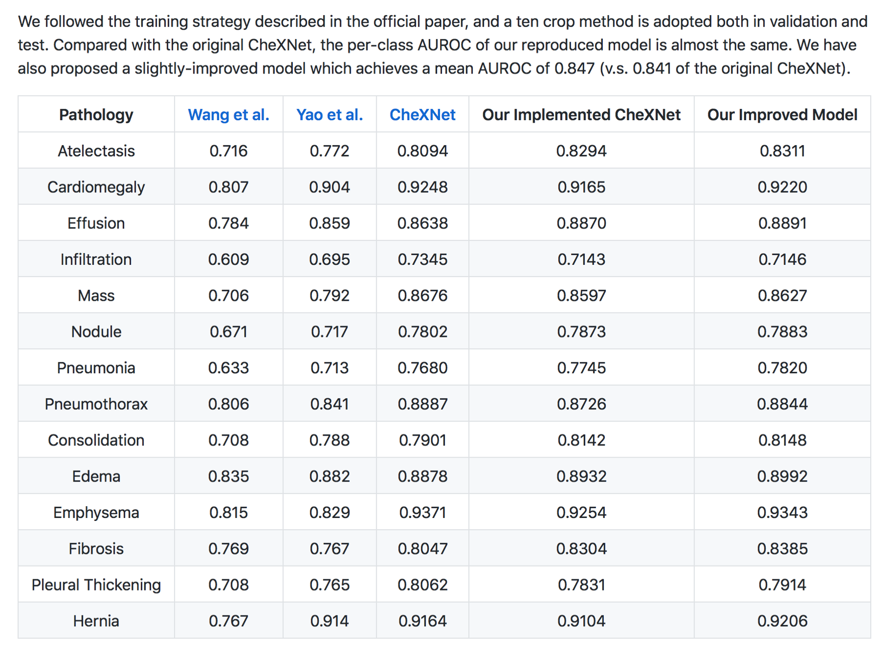
Moreover CheXNet has State of the Art (SOTA) performance on all 14 pathologies compared to prior publications.eval - prior benchmarks

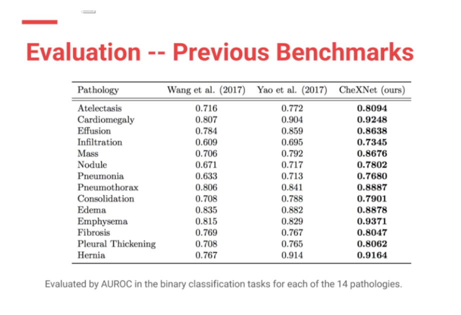
In my (JG) search , the Machine Intelligence Lab, Institute of Computer Science & Technology, Peking University, directed by Prof. Yadong Mu reports superior performance than the Stanford group. The code is open source and available here — https://github.com/arnoweng/CheXNet 

CheXNet, AUROC, ROC, n2value
Results from various implementations of ChexNet
Results from various implementations of ChexNet

Critique — Various studies that assess cognitive fit show that human performance can be affected by lack of clinical information or prior comparisons that may affect their performance. Moreover, before the most recent version of the paper, human performance was unfairly scored against the machine.

Clinical significance

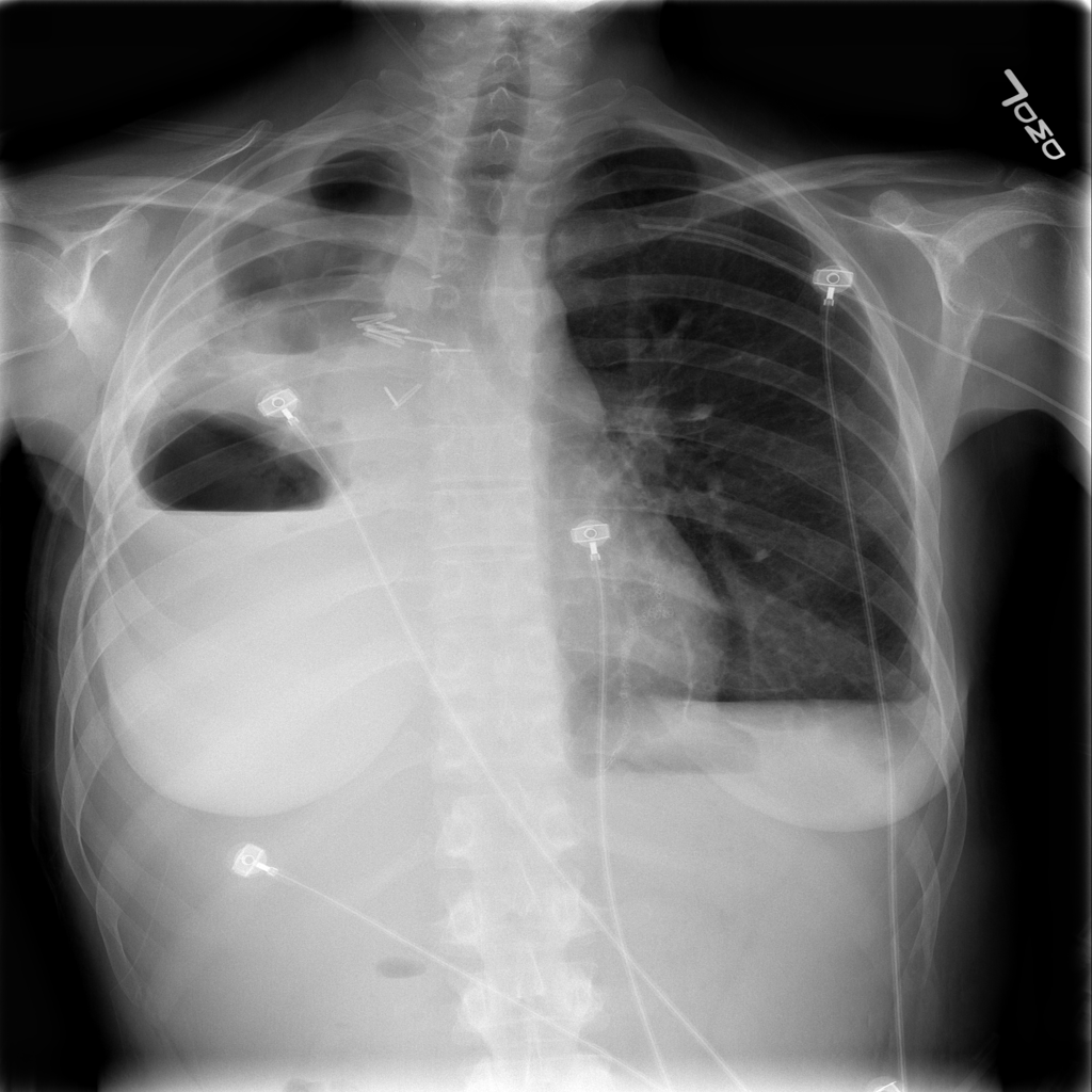
With the majority of labelled CXRs with pneumothorax having chest tubes present, the question must be raised: “are we training the Densenet to recognize pneumothoraces or chest tubes?”

Peer review

Luke Oakden-Rayner MD, a radiologist in Australia with expertise in AI & deep learning who was on our panel independently evaluated the ChestXRay-14 dataset, and CheXNet. He praises the Stanford team for their openness and patience in discussing the paper’s methodology, and their willingness to modify the paper to correct a methodologic flaw which biased against evaluating radiologists.

Summary

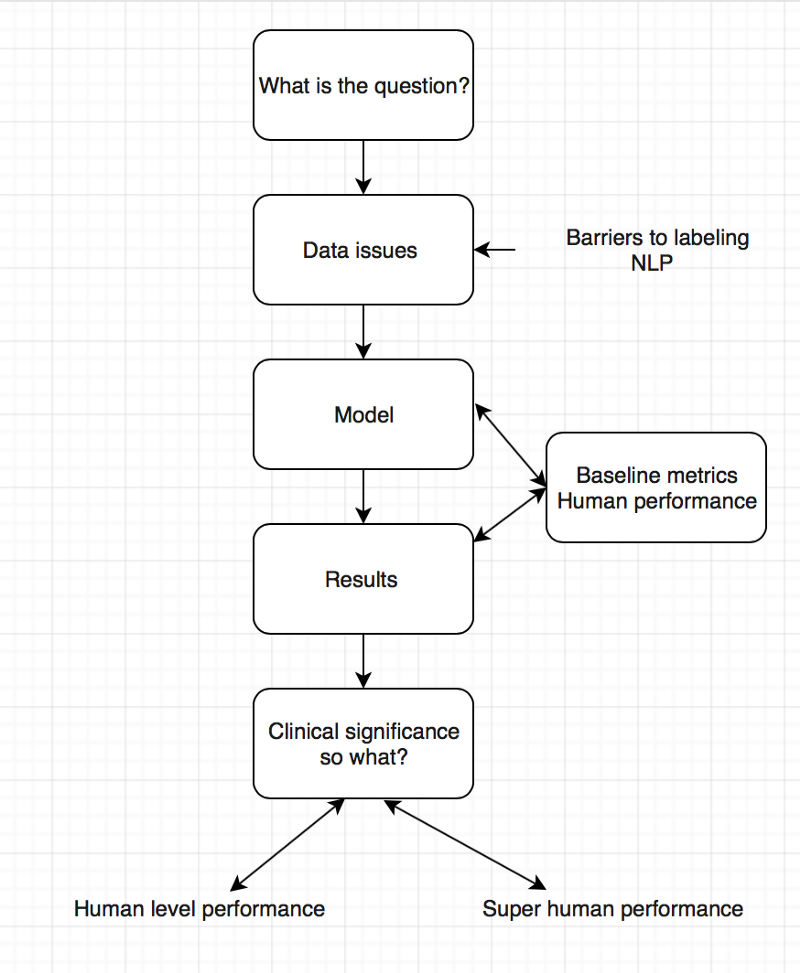
For the second AI journal club we analysed the pipeline of AI papers in medicine. You must make sure you are asking the right clinical question to be answered and not doing algorithms for the sake of doing something. Thereafter understand whether your data will help you answer the question you have, looking into details on how the data was collected and labeled.

To determine human level or super human performance, ensure the baseline metrics are adequate and not biased against one group.

Flowchart, AI, Deep Learning, Medicine, n2value
Pipeline for AI in medicine

The model appears to give at-human performance for experts, or better than human performance for less-trained practitioners. This is in line with research findings and Enlitic’s experience. We should not be surprised by that; the research in Convolutional Neural Networks has consistently reported near-human or super-human performance consistently.

Take Aways

  1. There is exists a critical gap in the labeling of medical data.
  2. Do not forget the clinical significance of your results.
  3. Embrace peer review especially in medicine and AI

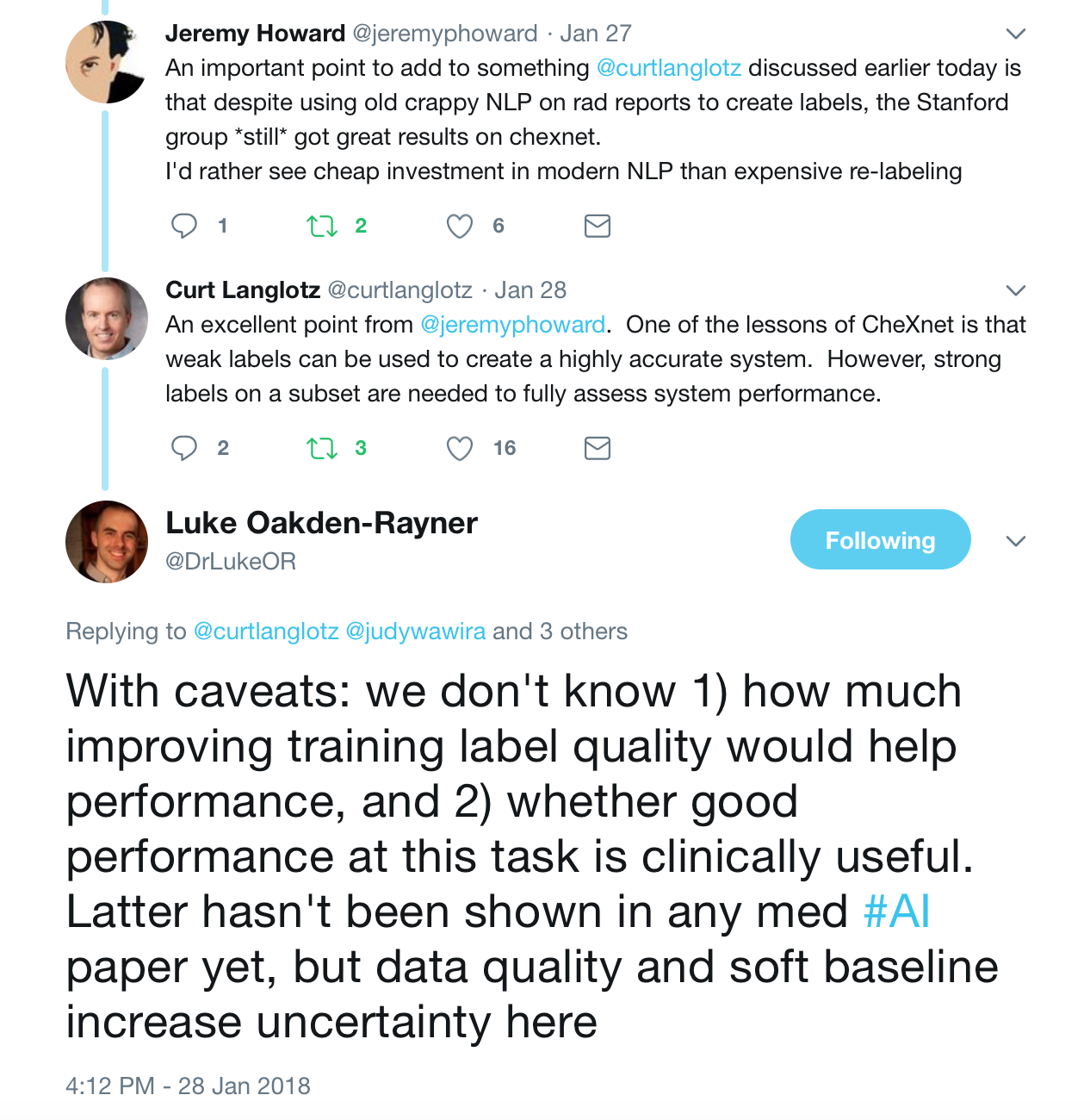
These were the best tweets regarding the problem of labeling medical data — aka do not get discouraged to attempt deep learning for medicine.

twitterJHKL

The journal club was a success, so if you are a doctor or an AI scientist , join us at https://tribe.radai.club to continue with the conversations on AI and medicine. You can listen to the recording of this journal club here : https://youtu.be/xoUpKjxbeC0 . Our next guest is Timnit Gebru who worked on US demographic household prediction using Google Street view images on 22nd February 2018. She will be talking on Using deep learning and Google Street View to estimate the demographic makeup of neighborhoods across the United States (http://www.pnas.org/content/114/50/13108).

Coming soon

For the journal club we developed a human versus AI competition for interepreting the CXRs in the dataset hosted at https://radai.club. We will be publishing the outcome of our crowdsourced labels soon, with a detailed analysis to check whether the model performance improves.

Say thanks

This I would like to thank the panelists including Jeremy Howard, Paras Lakhani, Luke Oakden-Rayner , and the Stanford ML team. Thanks to the ACR RFS AI advisory council members including Kevin Seals.

Article corrections made

  1. This article referred to Jeremy Howard (Ex-CEO of Kaggle) — updated to “president and chief scientist of Kaggle”
  2. Article stated NLP performance on that dataset is not likely improved over random.Jeremy clarified that the precision of the normal finding was what was not likely improved over random


OODA loop revisited – medical errors, heuristics, and AI.

OODA loop revisited – medical errors, heuristics, and AI.

My OODA loop post is actually one of the most popular on this site.   I  blame Venkatesh Rao of Ribbonfarm and his Tempo book and John Robb’s Brave New War for introducing me to Boyd’s methodology.   Venkatesh focuses on philosophy and management consulting, and Robb focuses on COIN and human social networks. Both are removed from healthcare, but applying Boyd’s principles to medicine: our enemy is disease, perhaps even ourselves.

Consider aerial dogfighting.  The human OODA loop is – Observe, Orient, Decide, Act.   You want to “get inside your opponent’s OODA loop” and out-think them, knowing their actions before they do, assuring victory.  If you know your opponent’s next move, you can anticipate where to shoot and end the conflict decisively.  Quoting Sun Tzu in The Art of War:

Sun Tzu Art of War OODA loops and AI

If you know the enemy and know yourself, you need not fear the result of a hundred battles. If you know yourself but not the enemy, for every victory gained you will also suffer a defeat. If you know neither the enemy nor yourself, you will succumb in every battle.

Focused, directed, lengthy and perhaps exhausting training for a fighter pilot enables them to “know their enemy” and anticipate action in a high-pressure, high-stakes aerial battle.  The penalty for failure is severe – loss of the pilot’s life.   Physicians prepare similarly – a lengthy and arduous training process in often adverse circumstances.  The penalty for failure is also severe – a patient’s death.  Given adequate intelligence and innate skill, successful pilots and physicians internalize their decision trees – transforming the OODA loop to a simpler OA loop – Observe and Act.  Focused practice allows the Orient and Decide portions of the loop to become automatic and intuitive, almost Zen-like.  This is what some people refer to as ‘Flow’ – an effortlessly hyperproductive state where total focus and immersion in a task suspends the perception of the passage of time.

For a radiologist, ‘flow’ is when you sit down at your PACS at 8am, continuously reading cases, making one great diagnosis after another, smiling as the words appear on Powerscribe. You’re killing the cases and you know it.  Then your stomach rumbles – probably time for lunch – you look up at the clock and it is 4pm.  That’s flow.

Flow is one of the reasons why experienced professionals are highly productive – and a smart manager will try to keep a star employee ‘in the zone’ as much as possible, removing extraneous interruptions, unnecessary low-value tasks, and distractions.

Kahneman defines this as fast type 1 thinking, intuitive and heuristic : quick, easy, and with sufficient experience/training, usually accurate.  But type 1 thinking can fail : a complex process masquerades as a simple one, additional important data is undiscovered or ignored, or a novel agent is introduced.  In these circumstances type 2 critical thinking is needed : slow, methodological, deductive and logical.  But humans err, substituting heuristic thinking for analytical thinking, and we get it wrong.

For the enemy fighter pilot, its the scene in Top Gun where Tom Cruise hits the air brakes to drop behind an attacking Mig to deliver a kill shot with his last missile. For a physician, it is an uncommon or rare disease presenting like a common one, resulting in a missed diagnosis and lawsuit.

To those experimenting in deep learning and Artificial intelligence, the time to train or teach the network far exceeds the time needed to process an unknown through the trained network.  Training can take hours to days, evaluation takes seconds.

Narrow AI’s like Convolutional Neural Networks take advantage of their speed to go through the OODA loop quickly, in a process called inference.  I suggest a deep learning algorithm functions as an OA loop on the specific type of data it has been trained on.  Inference is quick.

I believe that OODA loops are Kahneman’s Type 2 slow thinking.  OA loops are Kahneman’s Type 1 fast thinking.  Narrow AI inference is a type 1 OA loop.   An AI version of type 2 slow thinking doesn’t yet exist.*

And like humans, Narrow AI can be fooled.

Can your classifier tell the difference between a chihuahau and blueberry muffin?

If you haven’t seen the Chihuahua vs. blueberry muffin clickbait picture, consider yourself sheltered. Claims that narrow AI can’t tell the difference are largely, but not entirely, bogus.  While Narrow AI is generally faster than people, and potentially more accurate, it can still make errors. But so can people. In general, classification errors can be reduced by creating a more powerful, or ‘deeper’ network. I think collectively we have yet to decide how much error to tolerate in our AI’s. If we are willing to tolerate an error of 5% in humans, are we willing to tolerate the same in our AI’s, or do we expect 97.5%?  Or 99%? Or 99.9%?

The single pixel attack is a bit more interesting.  While similar images such as the ones above probably won’t pass careful human scrutiny, and frankly adversarial images unrecognizable to humans can be misinterpreted by a classifier:

Convolutional Neural Networks can be fooled by adversarial images

Selecting and perturbing a single pixel is much more subtle, and probably could escape human scrutiny.  Jaiwei Su et al address this in their “One Pixel Attack” paper, where the modification of one pixel in an image had between a 66% to 73% chance of changing the classification of that image.  By changing more than one pixel, success rates respectively rose.  The paper used older, less deep Narrow AI’s like VGG-16 and Network-in-network.  Newer models such as DenseNets and ResNets might be harder to fool.  This type of “attack” represents a real-world situation where the OA loop fails to account for unexpected new (or perturbed) information, and is incorrect.

Contemporaneous update: Google has developed images that use an adversarial attack to uniformly defeat classification attempts by standard CNN models.  By making “stickers” out of these processed images, the presence of such an image, even at less than 20% of the image size, is sufficient to change the classification to what the ensemble dictates, rather than the primary object in an image.  They look like this:

adversarial images capable of overriding CNN classifier
https://arxiv.org/pdf/1712.09665.pdf


I am not aware of defined solutions to these problems – the obvious images that fool the classifier can probably be dealt with by ensembling other, more traditional forms of computer vision image analysis such as HOG or SVM’s.  For a one-pixel attack, perhaps widening the network and increasing the number of training samples by either data augmentation or adversarially generated features might make the network more robust.  This probably falls into the “too soon to tell” category.

There has been a great deal of interest and emphasis placed lately on understanding black-box models.  I’ve written about some of these techniques in other posts.  Some investigators feel this is less relevant.  However, by understanding how the models fail, they can be strengthened.  I’ve also written about this, but from a management standpoint.  There is a trade off between accuracy at speed, robustness, and serendipity.  I think the same principle applies to our AI’s as well.  By understanding the frailty of speedy accuracy vs. redundancies that come at the expense of cost, speed, and sometimes accuracy, we can build systems and processes that not only work but are less likely to fail in unexpected & spectacular ways.

Let’s acknowledge the likelihood of failure of narrow AI where it is most likely to fail, and design our healthcare systems and processes around that, as we begin to incorporate AI into our practice and management.  If we do that, we will truly get inside the OODA loop of our opponent – disease – and eradicate it before it even had a chance.  What a world to live in where the only thing disease can say is, “I never saw it coming.”


*I believe OODA loops have mathematical analogues. The OODA loop is inherently Bayesian – next actions iteratively decided by prior probabilities. Iterative deep learning constructs include LSTM and RNN’s (Recurrent Neural Networks) and of course, General Adversarial Networks (GANs). There have been attempts to not only use Bayesian learning for hyperparameter optimization but also combining it with RL(Reinforcement Learning) & GANs.  Time will only tell if this brings us closer to the vaunted AGI (Artificial General Intelligence)**.

**While I don’t think we will soon solve the AGI question, I wouldn’t be surprised if complex combinations of these methods, along with ones not yet invented, bring us close to top human expert performance in a Narrow AI. But I also suspect that once we start coding creativity and resilience into these algorithms, we will take a hit in accuracy as we approach less narrow forms of AI.  We will ultimately solve for the best performance of these systems, and while it may even eventually exceed human ability, there will likely always be an error present.  And in that area of error is where future medicine will advance.

© 2018

n2value AI deep learning applied to chest x ray for radiology

CheXNet – a brief evaluation

Chest X-Ray deep dreamed - our AI & deep learning future
Chest Radiograph from ChestX-ray14 dataset processed with the deep dream algorithm trained on ImageNet

1/25/18: NOTE:  Since the November release of the CheXNet paper on ArXiV, there has been a healthy and extensive online discussion on twitter, reddit, and online blogs.  The Stanford paper has undergone at least two revisions with some substantial modifications, most importantly the replacement of ROC curves with F1 scores and a bootstrap calculation of significance.  Some details about the methodology which were not released in the original version have come out, particularly the “re-labeling” of ground truth by Stanford radiologists.  My comment about the thoracic specialist has completely borne out on further release of information. And the problems with ChestXRay14’s labeling (why the Stanford docs re-labeled) are now well-known.

The investigation and discussion of this paper has been spearheaded by Luke Oaken Rayner, who has spent months corresponding with the author and discussing the paper.  For further Information, see below.

The discussion on CheXNet appears to be over, and there has been a great deal of collective learning in it.  The Stanford group should be lauded for their willingness to engage in open peer review and modify their paper substantially after it.  There is no question that a typical 18-24 month process of review and discussion was fast-tracked in the last two months.  Relevant blog links are below after my December addendum.   This will be my last update on this post, as it is “not so brief” any longer!


Andrew Ng released CheXNet yesterday on ArXiv (citation) and promoted it with a tweet which caused a bit of a stir on the internet and related radiology social media sites like Aunt Minnie.  Before Radiologists throw away their board certifications and look for jobs as Uber drivers, a few comments on what this does and does not do.

First off, from the Machine Learning perspective, methodologies check out.  It uses a 121 layer DenseNet, which is a powerful convolutional neural network.  While code has not yet been provided, the DenseNet seems similar to code repositories online where 121 layers are a pre-made format.  80/20 split for Training/Validation seems pretty reasonable (from my friend, Kirk Borne), Random initialization, minibatches of 16 w/oversampling positive classes, and a progressively decaying validation loss are utilized, all of which are pretty standard.  Class activation mappings are used to visualize areas in the image most indicative of the activated class (in this case, pneumonia).  This is an interesting technique that can be used to provide some human-interpretable insights into the potentially opaque DenseNet.

The last Fully Connected (FC) layer is replaced by a single output (only one class is being tested for – pneumonia) coupled to a sigmoid function (an activation function – see here) to give a probability between 0 and 1.   Again, pretty standard for a binary classification.  The multiclass portion of the study was performed seperately/later.

The test portion of the study was 420 Chest X-rays read by four radiologists, one of whom was a thoracic specialist.  They could choose between the 14 pathologies in the ChestX-ray14 dataset, read blind without any clinical data.

So, a ROC curve was created, showing three radiologists similar to each other, and one outlier.The radiologists lie slightly under the ROC curve of the CheXNet classifier.  But, a miss is as good as a mile, so the claims of at or above radiologist performance are accurate, because math.  As Luke Oakden Rayner points out, this would probably not pass statistical muster.

So that’s the study.  Now, I will pick some bones with the study.

First, only including one thoracic radiologist is relevant, if you are going to make ground truth agreement of 3 out of four radiologists.  (Addendum: And, for statistical and methodological reasons discussed online, the 3 out of 4 implementation was initially flawed as scored)  General radiologists will be less specific than specialist radiologists, and that is one of the reasons why we have moved to specialty-specific reads over the last 20 years.  If the three general rads disagreed with the thoracic rad, the thoracic rad’s ground truth would be discarded.  Think about this – you would take the word of the generalist over the specialist, despite greater training.  (1/25 Addendum: proven right on this one.  The thoracic radiologist is an outlier with a higher F1 score)  Even Google didn’t do this in their retinal machine learning paper.  Instead, Google used their three retinal specialists as ground truth and then looked at how the non-specialty opthalmologists were able to evaluate that data and what it meant to the training dataset.  (Thanks, Melody!)  Nevertheless, all rads lie reasonably along the same ROC curve, so methodologically it checks out the radiologists are likely of equal ability but different sensitivities/specificities.

Second, the Wang ChestXray14 dataset is a dataset that was data-mined from NIH radiology reports.  This means that for the dataset, ground truth was whatever the radiologists said it was.  I’m not casting aspersions on the NIH radiologists, as I am sure they are pretty good.  I’m simply saying that the dataset’s ground truth is what it says it is, not necessarily what the patient’s clinical condition was.  As proof of that, here are a few cells from the findings field on this dataset.

Findings field from the ChestX-ray14 dataset (representative)

In any case, the NIH radiologists more than a few times perhaps couldn’t tell either, or identified one finding as the cause of the other (Infiltrate & Pneumonia mentioned side by side) and at the top you have the three fields “atelectasis” “consolidation” & “Pneumonia” – is this concurrent pneumonia with consolidation with some atelectasis elsewhere, or is it “atelectasis vs consolidation cannot r/o pneumonia” (as radiologists we say these things). While the text miner purports to use several advanced NLP tools to avoid these kinds of problems, in practice it does not seem to do so. (See addendum below, further addendum, confirmed by Jeremy Howard)  Dr. Ng, if you read this, I have the utmost respect for you and your team, and I have learned from you.  But I would love to know your rebuttal, and I would urge you to publish those results.  Or perhaps someone should do it for reproducibility purposes.

Finally, I’m bringing up these points not to be a killjoy, but to be balanced.  I think it is important to see this and prevent someone from making a really boneheaded decision of firing their radiologists to put in a computer diagnostic system (not in the US, but elsewhere) and realizing it doesn’t work after spending a vast sum of money on it.  Startups competing in the field who do not have deep healthcare experience need to be aware of potential pitfalls in their product.  I’m saying this because real people could be really hurt and impacted if we don’t manage this transition into AI well.  Maybe all parties involved in medical image analysis should join us in taking the Hippocratic Oath, CEO’s and developers included.

Thanks for reading, and feel free to comment here or on twitter or connect on linkedin to me: @drsxr

December Addendum: ChestX-ray14 is based on the ChestX-ray8 database which is described in a paper released on ArXiv by Xiaosong Wang et al. The text mining is based upon a hand-crafted rule-based parser using weak labeling designed to account for “negation & uncertainty”, not merely application of regular expressions. Relationships between multiple labels are expressed, and while labels can stand alone, for the label ‘pneumonia’, the most common associated label is ‘infiltrate’.  A graph showing relationships between the different labels in the dataset is here (from Wang Et Al.)

Label map from the ChestX-ray14 dataset by Wang et. al.

Pneumonia is purple with 2062 cases, and one can see the largest association is with infiltration, then edema and effusion.  A few associations with atelectasis also exist (thinner line).

The dataset methodology claims to account for these issues at up to 90% precision reported in ChestX-ray8, with similar precision inferred in ChestX-ray14.

No Findings (!) from NIH CXR14 dataset
“No Findings”
No Findings (!) from NIH CXR14 Dataset
“No Findings”

However, expert review of the dataset (ChestX-ray14) does not support this.  In fact, there are significant concerns that the labeling of the dataset is a good deal weaker.  I’ll just pick out two examples above that show a patient likely post R lobectomy with attendant findings classified as “No Findings” and the lateral chest X-ray which doesn’t even belong in the study database of all PA and AP films.  These sorts of findings aren’t isolated – Dr. Luke Oakden-Rayner addresses this extensively in this post, from which his own observations are garnered below:

Sampled PPV for ChestX-Ray14 dataset vs reported
Dr. Luke Oakden Rayner’s own Positive Predictive Value on visual inspection of 130 images vs reported

His final judgment is that the ChestX-ray14 dataset is not fit for training medical AI systems to do diagnostic work.  He makes a compelling argument, but I think it is primarily a labelling problem, where the proposed 90% acccuracy on the NLP data mining techniques of Wang et al does not hold up.  ChestX-ray14 is a useful dataset for the images alone, but the labels are suspect.  I would call upon the NIH group to address this and learn from this experience.  In that light, I am surprised that the system did not do a great deal better than the human radiologists involved in Dr. Ng’s group’s study, and I don’t really have a good explanation for it.

The evaluation of CheXNet by these individuals should be recognized:

Luke Oakden-Rayner: CheXNet an in-depth review

Paras Lakhani : Dear Mythical Editor: Radiologist-level Pneumonia Detection in CheXNet

Bailint Botz: A Few thoughts about ChexNet

Copyright © 2017

Building a high-performance GPU computing workstation for deep learning – part I

This post is cross posted to www.ai-imaging.org .  For machine learning and AI issues, please visit the new site!

With Tensorflow released to the public, the NVidia Pascal Titan X GPU, along with (relatively) cheap storage and memory, the time was right to take the leap from CPU-based computing to GPU accelerated machine learning.

My venerable Xeon W3550 8GB T3500 running a 2GB Quadro 600 was outdated. Since a DGX-1 was out of the question ($129,000), I decided to follow other pioneers building their own deep learning workstations. I could have ended up with a multi-thousand dollar doorstop – fortunately, I did not.

Criteria:

  1. Reasonably fast CPU
  2. Current ‘Best’ NVidia GPU with large DDR5 memory
  3. Multi-GPU potential
  4. 32GB or more stable RAM
  5. SSD for OS
  6. Minimize internal bottlenecks
  7. Stable & Reliable – minimize hardware bugs
  8. Dual Boot Windows 10 Pro & Ubuntu 16.04LTS
  9. Can run: R, Rstudio, Pycharm, Python 3.5, Tensorflow


Total:                                                 $3725


Asus X99 E 10G WS Motherboard. Retail $699

A Motherboard sets the capabilities and configuration of your system. While newer Intel Skylake and Kaby Lake CPU architectures & chipsets beckon, reliability is important in a computationally intensive build, and their documented complex computation freeze bug makes me uneasy. Also, both architectures remain PCIe 3.0 at this time.

Therefore, I chose the ASUS X99 motherboard. The board implements 40 PCIe 3.0 lanes which will support three 16X PCIe 3.0 cards (i.e. GPU’s) and one 8x card. The PCIe 3.0-CPU lanes are the largest bottleneck in the system, so making these 16X helps the most.  It also has a 10G Ethernet jack somewhat future-proofing it as I anticipate using large datasets in the Terabyte size. It supports up to 128GB of DDR4. The previous versions of ASUS X99 WS have been well reviewed.


Intel Core i7 6850K Broadwell-E CPU Socket Retail $649

Socket LGA2011-v3 on the motherboard guides the CPU choice – the sweet spot in the Broadwell-E lineup is the overclockable 3.6Ghz 6850K with 6 cores and 15MB of L3 cache, permitting 40 PCIe lanes. $359 discounted is attractive compared to the 6900K, reviewed to offer minimal to no improvement at a $600 price premium. The 6950X is $1200 more for 4 extra cores, unnecessary for our purposes. Avoid the $650 6800K – pricier and slower with less (28) lanes. A stable overclock to 4.0Ghz is easily achievable on the 6850K.

NVidia GeForce 1080Ti 11GB – EVGA FTW3 edition Retail: $800

Last year, choosing a GPU was easy – the Titan X Pascal, a 12GB 3584 CUDA-core monster. However, by spring 2017 there were two choices: The Titan Xp, with slightly faster memory speed & internal bus, and 256 more CUDA cores; and the 1080Ti, the prosumer enthusiast version of the Titan X Pascal, with 3584 cores. The 1080Ti differs in its memory architecture – 11GB DDR5 and a slightly slower, slightly narrower bandwidth vs. the Xp.

The 1080Ti currently wins on price/performance. You can buy two 1080Ti’s for the price of one Titan Xp. Also, at time of purchase, Volta architecture was announced. As the PCIe bus is the bottleneck, and will remain so for a few years, batch size into DDR5 memory & CUDA cores will be where performance is gained. A 16GB DDR5 Volta processor would be a significant performance gain from a 12GB Pascal for deep learning. Conversely, 12GB Pascal to 11GB Pascal is a relative lesser performance hit. As I am later in the upgrade cycle, I’ll upgrade to the 16GB Volta and resell my 1080Ti in the future – I anticipate only taking a loss of $250 per 1080Ti on resell.

The FTW3 edition was chosen because it is a true 2-slot card (not 2.5) with better cooling than the Founder’s Edition 1080Ti. This will allow 3 to physically fit onto this motherboard.

64 GB DDR4-2666 DRAM – Corsair Vengeance low profile Retail : $600

DDR4 runs at 2133mhz unless overclocked. Attention must be paid to the size of the DRAM units to ensure they fit under the CPU cooler, which these do. From my research, DRAM speeds over 3000 lose stability. For Broadwell there’s not much evidence that speeds above 2666mhz improves performance. I chose 64GB because 1) I use R which is memory resident so the more GB the better and 2) There is a controversial rule of thumb that your RAM should equal 2x the size of your GPU memory to prevent bottlenecks. Implementing 3 1080Ti’s, 3x 11GB = 33 GB. Implementing 2 16GB Voltas would be 32GB.


Samsung 1TB 960 EVO M2 NVMe SSD Retail $500

The ASUS motherboard has a fast M2 interface, which, while using PCIe lanes, does not compete for slots or lanes. The 1TB size is sufficient for probably anything I will throw at it (all apps/programs, OS’s, and frequently used data and packages. Everything else can go on other storage. I was unnecessarily concerned about SSD heat throttling – on this motherboard, the slot’s location is in a good place which allows for great airflow over it. The speed in booting up Windows 10 or Ubuntu 16.04 LTS is noticeable.


EVGA Titanium 1200 power supply Retail $350

One of the more boring parts of the computer, but for a multi GPU build you need a strong 1200 or 1600W power supply. The high Titanium rating will both save on electricity and promote stability over long compute sessions.


Barracuda 8TB Hard Drive Retail $299

I like to control my data, so I’m still not wild about the cloud, although it is a necessity for very large data sets. So here is a large, cheap drive for on-site data storage. For an extra $260, I can Raid 1 the drive and sleep well at night.

Strike FUMA CPU Cooler. Retail $60

This was actually one of the hardest decisions in building the system – would the memory will fit under the fans? The answer is a firm yes. This dual fan tower cooler was well-rated, quiet, attractive, fit properly, half the price of other options, and my overclocked CPU runs extremely cool – 35C with full fan RPM’s, average operating temperature 42C and even under a high stress test, I have difficulty getting the temperature over 58C. Notably, the fans never even get to full speed on system control.


Corsair 750 D Airflow Edition Case. Retail $250

After hearing the horror stories of water leaks, I decided at this level of build not to go with water cooling. The 750D has plenty of space (enough for a server) for air circulation, and comes installed with 3 fans – two air intake on the front and one exhaust at upper rear. It is a really nice, sturdy, large case. My front panel was defective – the grating kept falling off – so Corsair shipped me a replacement quickly and without fuss.

Cougar Vortex 14” fans – Retail $20 ea.

Two extra cougar Vortex 14” fans were purchased, one as an intake fan at the bottom of the case, and one as a 2nd exhaust fan at the top of the case. These together create excellent airflow at noise levels I can barely hear. Two fans on the CPU Heat Sink plus Three Fans on the GPU plus five fans on the case plus one in the power supply = 11 fans total! More airflow at lower RPM = silence.


Windows 10 Pro USB edition Retail $199

This is a dual boot system so, there you go.

Specific limitations with this system are as follows. While it will accept four GPU’s physically, the slots are limited to 16X/16X/16X/8X with the M2 drive installed which may affect performance on the 4th GPU (& therefore deep learning model training and performance). Additionally, the CPU upgrade path is limited – without going to a Xeon, the only reasonable upgrade from the 6850K’s 14,378 passmark is the 6950X, with a passmark of 20,021. In the future if more than 128GB DDR4 is required, that will be a problem with this build.

Finally, inherent bandwidth limitations exist in the PCIe 3.0 protocol and aren’t easily circumvented. PCIe 3.0 throughput is 8GB/s. Compare this to NVidia’s proprietary NVlink that allows throughput of 20-25GB/s (Pascal vs. Volta). Note that current NVlink speeds will not be surpassed until PCIe5.0 is implemented at 32GB/s in 2019. NVidia’s CUDA doesn’t implement SLI, either, so at present that is not a solution. PCIe 4.0 has just been released with only IBM adopting, doubling transfer vs. 3.0, and 5.0 has been proposed, doubling yet again. However, these faster protocols may be difficult and/or expensive to implement. A 4 slot PCIe 5.0 bus will probably not be seen until into the 2020’s. This means that for now, dedicated NVlink 2.0 systems will outperform similar PCIe systems.

With that said, this system approaches a best possible build considering price and reliability, and should be able to give a few years of good service, especially if the GPU’s are upgraded periodically. Precursor systems based upon the Z97 chipset are still viable for deep learning, albeit with slower speeds, and have been matched to older NVidia 8GB 1070 GPU’s which are again half the price of the 1080Ti.

In part II, I will describe how I set up the system configuration for dual boot and configured deep learning with Ubuntu 16.04LTS. Surprisingly, this was far more difficult than the actual build itself, for multiple reasons I will explain & detail with the solutions.  And yes, it booted up.  On the first try.

If you liked this post, head over to our sister site, ai-imaging.org where part 2, part 3, and part 4 of this post are located.

Machine Intelligence in Medical Imaging Conference – Report

blueI heard about the Society of Imaging Informatics in Medicine’s (SIIM) Scientific Conference on Machine Intelligence in Medical Imaging (C-MIMI) on Twitter.  Priced attractively, easy to get to, I’m interested in Machine Learning and it was the first radiology conference I’ve seen on this subject, so I went.  Organized on short notice so I was expecting a smaller conference.

cmimipacked

I almost didn’t get a seat.  It was packed.

The conference had real nuts and bolts presentations & discussions on healthcare imaging machine learning (ML).  Typically, these were Convolutional Neural Networks (CNN‘s/Convnets) but a few Random Forests (RF) and Support Vector Machines (SVM) sneaked in, particularly in hybrid models along with a CNN (c.f.  Microsoft).  Following comments assume some facility in understanding/working with Convnets.

Some consistent threads throughout the conference:

  • Most CNN’s were trained on Imagenet with the final fully connected (FC) layer removed; then re-trained on radiology data with a new classifer FC layer placed at the end.
  • Most CNN’s were using Imagenet standard three layer RGB input despite being greyscale.  This is of uncertain significance and importance.
  • The limiting of input matrices to grids less than image size is inherited from the Imagenet competitions (and legacy computational power).  Decreased resolution is a limiting factor in medical imaging applications, potentially worked-around by multi-scale CNN’s.
  • There is no central data repository for a good “Ground Truth” to develop improved machine imaging models.
  • Data augmentation methods are commonly used due to lower numbers of obtained cases.

Keith Dryer DO PhD gave an excellent lecture about the trajectory of machine imaging and how it will be an incremental process with AI growth more narrow in scope than projected, chiefly limited by applications.  At this time, CNN creation and investigation is principally an artisanal product with limited scalability.  There was a theme – “What is ground truth?” which in different instances is different things (path proven, followed through time, pathognomonic imaging appearance).

There was an excellent educational session from the FDA’s Berkman Sahiner.  The difference between certifying a type II or type III device may keep radiologists working longer than expected!  A type II device, like CAD, identifies a potential abnormality but does not make a treatment recommendation and therefore only requires a 510(k) application.  A type III device, as in an automated interpretation program creating diagnosis and treatment recommendations will require a more extensive application including clinical trials, and a new validation for any material changes.  One important insight (there were many) was that the FDA requires training and test data to be kept separate.   I believe this means that simple cross-validation is not acceptable nor sufficient for FDA approval or certification.  Adaptive systems may be a particularly challenging area for regulation, as similar to the ONC, significant changes to the software of the algorithm will require a new certification/approval process.

Industry papers were presented from HK Lau of Arterys, Xiang Zhou of Siemens, Xia Li of GE, and Eldad Elnekave of Zebra medical.  The Zebra medical presentation was impressive, citing their use of the Google Inception V3 model and a false-color contrast limited adaptive histogram equalization algorithm, which not only provides high image contrast with low noise, but also gets around the 3-channel RGB issue.  Given statistics for their CAD program were impressive at 94% accuracy compared to a radiologist at 89% accuracy.

Scientific Papers were presented by Matthew Chen, Stanford; Synho Do, Harvard; Curtis Langlotz, Stanford; David Golan, Stanford; Paras Lakhani, Thomas Jefferson; Panagiotis Korfiatis, Mayo Clinic; Zeynettin Akkus, Mayo Clinic; Etka Bullar, U Saskatchewan; Mahmudur Rahman, Morgan State U; Kent Ogden SUNY upstate.

Ronald Summers, MD PhD from the NIH gave a presentation on the work from his lab in conjunction with Holger Roth, detailing the specific CNN approaches to Lymph Node detection, Anatomic level detection, Vertebral body segmentation, Pancreas Segmentation, and colon polyp screening with CT-colonography, which had high False Positives.  In his experience, deeper models performed better.  His lab also changes unstructured radiology reporting into structured reporting through ML techniques.

Abdul Halabi of NVIDIA gave an impressive presentation on the supercomputer-like DGX-1 GPU cluster (5 deliveries to date, the fifth of which was to Mass. General, a steal at over $100K), and the new Pascal architecture in the P4 & P40 GPU’s.  60X performance on AlexNet vs the original version/GPU configuration in 2012.  Very impressive.

Sayan Pathak of Microsoft Research and the Inner Eye team gave a good presentation where he demonstrated that a RF was really just a 2 layer DNN, i.e. a sparse 2 layer perceptron.   Combining this with a CNN (dNDE.NET), it beat googLENet’s latest version in the Imagenet arms race.  However, as one needs to solve for both structures simultaneously, it is an expensive (long, intense) computation.

Closing points were the following:

  • Most devs currently using Python – Tensorflow +/- Keras with fewer using CAFFE off of  Modelzoo
  • DICOM -> NIFTI -> DICOM
  • De-identification of data is a problem, even moreso when considering longitudinal followup.
  • Matching accuracy to the radiologist’s report may not be as important as actual outcomes report.
  • There was a lot of interest in organizing a competition to advance medical imaging, c.f. Kaggle.
  • Radiologists aren’t obsolete just yet.

It was a great conference.  An unexpected delight.  Food for your head!


Memory requirements for Convolutional Neural Network analysis of brain MRI.

Believed to be in the publc domainI’m auditing the wonderful Stanford CS 231n class on Convolutional Neural Networks in Computer Vision.

A discussion the other day was on the amount of memory required to analyze one image as it goes through the Convolutional Neural Network (CNN). This was interesting – how practical is it for application to radiology imaging?  (To review some related concepts see my earlier post : What Big Data  Visualization Analytics can learn from Radiology)

Take your standard non-contrast MRI of the brain. There are 5 sequences (T1, T2, FLAIR, DWI, ADC). For the purposes of this analysis, all axial. Assume a 320×320 viewing matrix for each slice. Therefore, one image will be a 320x320x5 matrix suitable for processing into a 512,000 byte vector. Applying this to the VGGNet Protocol D (1) yields the following:

VGGNet

In each image, there are 320 x and y pixels and each pixel holding a greyscale value. There are 5 different sequences. Each axial slice takes up 512KB, the first convolutional layers hold most of the memory at 6.4MB each, and summing all layers uses 30.5MB. Remember that you have to double the memory for the forward/backward pass through the network, giving you 61MB per image. Finally, the images do not exist in a void, but are part of about 15 axial slices of the head, giving you a memory requirement of 916.5MB, or about a gigabyte.

Of course, that’s just for feeding an image through the algorithm.

This is simplistic because:

  1. VGG is not going to get you to nearly enough accuracy for diagnosis! (50% accurate, I’m guessing)
  2. The MRI data is only put into slices for people to interpret – the data itself exists in K-space. What that would do to machine learning interpretation is another discussion.
  3. We haven’t even discussed speed of training the network.
  4. This is for older MRI protocols.  Newer MRI’s have larger matrices (512×512) and thinner slices (3mm) available, which will increase the necessary memory to approximately 4GB.

Nevertheless, it is interesting to note that the amount of memory required to train a neural network of brain MRI’s is in reach of a home network enthusiast.

(1). Karen Simonyan & Andrew Zisserman, Very Deep Convolutional Networks for Large-Scale Visual Recognition, ICLR 2015

The coming computer vision revolution

3 layer (7,5,3 hidden layers) neural network created in R using the neuralnet package.


Nothing of him that doth fade
But doth suffer a sea-change
Into something rich and strange.

– Shakespeare, The Tempest 1.2.396-401

I’m halfway through auditing Stanford’s CS231n course – Convolutional Neural Networks for Visual Recognition.

Wow. Just Wow. There is a sea-changing paradigm shift that is happening NOW –  we probably have not fully realized it yet.

We are all tangentially aware of CV applications in our daily lives – Facebook’s ability to find us in photos, optical character recognition (OCR) of our address on postal mail, that sort of thing. But these algorithms were rule-based expert systems grounded in supervised learning methods. Applications were largely one-off for a specific, single task. They were expensive, complicated, and somewhat error prone.

So what changed?   First, a little history. In the early 1980’s I had a good friend obtaining a MS in comp sci all atwitter about “Neural Networks”. Back then they went nowhere. Too much processing/memory/storage required, too difficult to tune, computationally slow. Fail.

Then:

1999 –  Models beginning with SIFT & ending with SVM (support vector machine) deformable parts. Best model only 74% accurate.

2006 – Restricted Boltzmann Machines apply backpropogation to allow deep neural networks.

2012 – AlexNet Deep learning applied to Imagenet classification database competition achieves a nearly 2X increase in accuracy to earlier SVM methods.

2015-   ResNet Deep learning system achieves a 4.5X increase in accuracy compared to Alexnet and 8X increase in accuracy to old SVM models.

In practical aspects, what does this mean? On a data set with 1000 different items  (ImageNet), ResNet is getting the item 100% correct (compared to a human) about 80% of the time, and correctly classifies the image as one of a list of 5 most probable items 96.4% of the time. People are typically believed to have 95% accuracy identifying the correct image. It’s clear to see that the computer is not far off.

2012 was the watershed year with the first application and win of the CNN to the dataset, and the improvement was significant enough it sparked additional refinements and development. That is still going on – the ResNet example was just released in December 2015! It’s clear that this is an area of active research and further improvements expected.

The convolutional neural network is a game-changer and will likely approach and perhaps exceed human accuracy in computer vision and classification in the near future. That’s a big deal.  As this is a medical blog, the applications to healthcare are obvious – radiology, pathology, dermatology, ophthalmology for starters.  But the CNN may also be useful for the complicated process problems I’ve developed here on the blog – the flows themselves resemble networks naturally.  So why not model them as such?  Why is it a game changer?  Because the model is probably universally adaptable to visual classification problems and once trained, potentially cheap.


I’ll  write more on this in the coming weeks – I’ve been inching towards deep learning models (but lagging blogging about them) but there is no reason to wait any more. The era of the deep learning neural network is here.