Developing a simple care delivery model further – dependent interactions

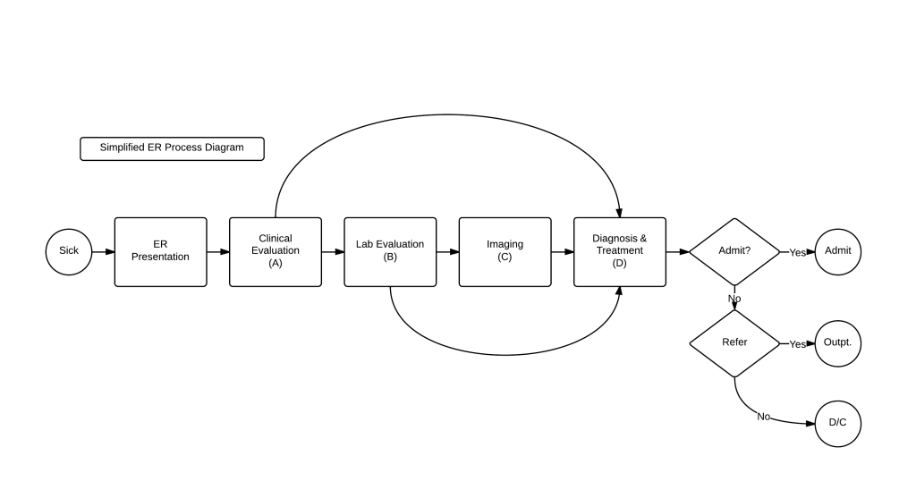
Let’s go back to our simple generalized linear model of care delivery from this post:

With its resultant Generalized Linear Function:

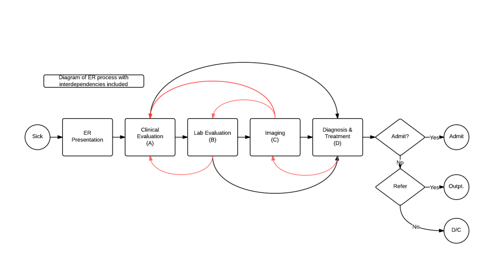
This model, elegant in its simplicity, does not account for the inter-dependencies in care delivery.  A more true-to-life revised model is:

Where there are options for back and forth pathways depending on new clinical information, denoted in red.

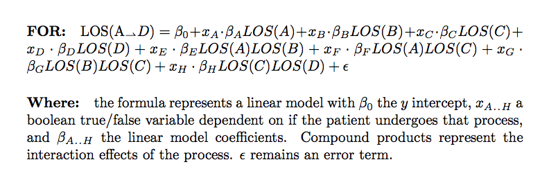
A linear model that takes into account these inter-dependencies would look like this:

Including these interactions, we go from 4 terms to 8.  And this is a overly-simplified model!  By drilling down in a typical PI/Six Sigma environment into an aspect of the healthcare delivery processes, its not hard to imagine creating well over four points of contact/patient interaction, each with their own set of interdependencies.  Imagine a process with 12-15 sub-processes and most of those sub-processes each having on average six (6) interdependencies.  And then the possibility of multiple interdependencies among the processes…  This doesn’t even account for a EMR dataset where the number of columns could be …. 350?  Quickly, your ‘simple’ linear model is looking not so simple with easily over 100 terms in the equation, which also causes solvation problems.     Not to despair!  There are ways to take this formula with a high number of terms and create a more manageable model as a reasonable approximation!  The mapping and initial modeling of the care process is of greatest utility from an operational standpoint, to allow for understanding and to guide interpretation of the ultimate data analysis.

I am a believer that statistical computational analysis can identify the terms which are most important for the model.  By inference, these inputs will have the most effect upon outcome, and can guide management to where precious effort, resources, and time should be guided to maximize outcomes.