Returning to our care model that discussed in parts one and two, we can begin by defining our variables.
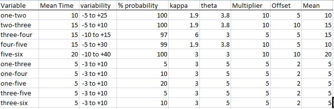
Each sub-process variable is named for its starting sub-process and ending sub-process. We will define mean time for the sub-processes in minutes, and add a component of time variability. You will note that the variability is skewed – some shorter times exist, but disproportionately longer times are possible. This coincides with real-life: in a well-run operation, mean times may be close to lower limits – as these represent physical (occurring in the real world) processes, there may simply be a physical constraint on how quickly you can do anything! However, problems, complications and miscommunications may extend that time well beyond what we all would like it to be – for those of us who have had real-world hospital experience, does this not sound familiar?
Because of this, we will choose a gamma distribution to model our processes:
 = \int_{0}^{\infty} {t^{a-1}e^{-t}dt}")
The gamma distribution is useful because it deals with continuous time data, and we can skew it through its shaping parameters Kappa (

It is generally recognized that a probability density plot (or Kernel plot) as opposed to a histogram of distributions is more accurate and less prone to distortions related to number of samples (N). A plot of these distributions looks like this: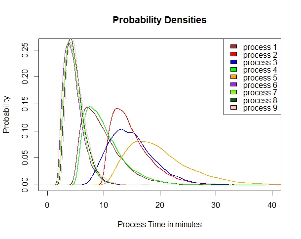
The R code to generate this distribution, graph, and our initial values dataframe is as follows:
seed <- 3559
set.seed(seed,kind=NULL,normal.kind = NULL)
n <- 16384 ## 2^14 number of samples then let’s initialize variables
k <- c(1.9,1.9,6,1.9,3.0,3.0,3.0,3.0,3.0)
theta <- c(3.8,3.8,3.0,3.8,3.0,5.0,5.0,5.0,5.0)
s <- c(10,10,5,10,10,5,5,5,5,5)
o <- c(4.8,10,5,5.2,10,1.6,1.8,2,2.2)
prosess1 <- (rgamma(n,k[1],theta[1])*s[1])+o[1]
prosess2 <- (rgamma(n,k[2],theta[2])*s[2])+o[2]
prosess3 <- (rgamma(n,k[3],theta[3])*s[3])+o[3]
prosess4 <- (rgamma(n,k[4],theta[4])*s[4])+o[4]
prosess5 <- (rgamma(n,k[5],theta[5])*s[5])+o[5]
prosess6 <- (rgamma(n,k[6],theta[6])*s[6])+o[6]
prosess7 <- (rgamma(n,k[7],theta[7])*s[7])+o[7]
prosess8 <- (rgamma(n,k[8],theta[8])*s[8])+o[8]
prosess9 <- (rgamma(n,k[9],theta[9])*s[9])+o[9]
d1 <- density(prosess1, n=16384)
d2 <- density(prosess2, n=16384)
d3 <- density(prosess3, n=16384)
d4 <- density(prosess4, n=16384)
d5 <- density(prosess5, n=16384)
d6 <- density(prosess6, n=16384)
d7 <- density(prosess7, n=16384)
d8 <- density(prosess8, n=16384)
d9 <- density(prosess9, n=16384)
plot.new()
plot(d9, col=”brown”, type = “n”,main=”Probability Densities”,xlab = “Process Time in minutes”, ylab=”Probability”,xlim=c(0,40), ylim=c(0,0.26))
legend(“topright”,c(“process 1″,”process 2″,”process 3″,”process 4″,”process 5″,”process 6″,”process 7″,”process 8″,”process 9”),fill=c(“brown”,”red”,”blue”,”green”,”orange”,”purple”,”chartreuse”,”darkgreen”,”pink”))
lines(d1, col=”brown”, add=TRUE)
lines(d2, col=”red”, add=TRUE)
lines(d3, col=”blue”, add=TRUE)
lines(d4, col=”green”, add=TRUE)
lines(d5, col=”orange”, add=TRUE)
lines(d6, col=”purple”, add=TRUE)
lines(d7, col=”chartreuse”, add=TRUE)
lines(d8, col=”darkgreen”, add=TRUE)
lines(d9, col=”pink”, add=TRUE)
ptime <- c(d1[1],d2[1],d3[1],d4[1],d5[1],d6[1],d7[1],d8[1],d9[1])
pdens <- c(d1[2],d2[2],d3[2],d4[2],d5[2],d6[2],d7[2],d8[2],d9[2])
ptotal <- data.frame(prosess1,prosess2,prosess3,prosess4,prosess5,prosess6,prosess7,prosess8,prosess9)
names(ptime) <- c(“ptime1″,”ptime2″,”ptime3″,”ptime4″,”ptime5″,”ptime6″,”ptime7″,”ptime8″,”ptime9”)
names(pdens) <- c(“pdens1″,”pdens2″,”pdens3″,”pdens4″,”pdens5″,”pdens6″,”pdens7″,”pdens8″,”pdens9”)
names(ptotal) <- c(“pgamma1″,”pgamma2″,”pgamma3″,”pgamma4″,”pgamma5″,”pgamma6″,”pgamma7″,”pgamma8″,”pgamma9”)
pall <- data.frame(ptotal,ptime,pdens)
Where the relevant term is rgamma(n,
One last concept needs to be discussed: The probability of the sub-processes’ occurence. Each sub-process has a percentage chance of happening – some a 100% certainty, others a fairly low 5% of cases. This reflects the real world reality of what happens – once a test is ordered, there’s a 100% certainty of the patient showing up for the test, but not 100% of the patients will get the test. Some cancel due to contraindications, others can’t tolerate it, others refuse, etc… The percentages that are <100% reflect those probabilities and essentially are like a non-binary boolean switch applied to the beginning of the term that describes that sub-process. We’re evolving first toward a simple generalized linear equation similar to that put forward in this post. I think its going to look somewhat like this:
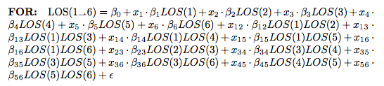 But we’ll see how well this model fares as we develop it and compare it to some others. The x terms will likely represent the probabilities between 0 and 1.0 (100%).
For a EMR based approach, we would assign a UID (medical record # plus 5-6 extra digits, helpful for encounter #’s). We will ‘disguise’ the UID by adding or subtracting a constant known only to us and then performing a mathematical operation on it. However, for our purposes here, we would not need to do that.
We’ll head on to our analysis in part 4.
Programming notes in R:
1. I experimented with for loops and different configurations of apply with this, and after a few weeks of experimentation, decided I really can’t improve upon the repetitive but simple code above. The issue is that the density function returns a list of 7 variables, so it is not as easy as defining a matrix, as the length of the data frame changes. I’m sure there is a way to get around this, but for the purposes of this illustration it is beyond our needs. Email me at mailto:contact@n2value.com if you have working code that does it better!
2. For the density function, the number of samples must be a power of 2. So by choosing 16384 (2^14) we meet that goal. Setting N to that number makes the data frame more symmetric.
3. In variable names above, prosess is an intentional misspelling.